Monday, 22 December 2014

(UPSC Economics Optional 2014) Question 7

"Monetarists are of the view that only money matters and Keynesians believe that money does not matter at all". What is the reasoning behind these extreme views held by their protagonists?

Key differences between these two schools:

MonetaristsKeynesians
Tie monetary policy to rulesGive policymakers discretion.
Fiscal policy is not useful.Fiscal policy may be useful.
AS curve has a steep slope.
Economy is inherently stable.
Economy can be unstable.
AS curve can be flat.

Detailed debate between monetarists and Keynesians: www.tcd.ie/Economics/assets/pdf/SER/1994/Alan_Dunne.html

(UPSC Economics Optional 2014) Question 6:

Discuss the cobweb model of dynamic equilibrium with lagged adjustment. Explain how the existence of a stable equilibrium depends on the nature of the demand and supply curves. (20 marks)

Part one:
Dynamic Stabiltiy: Dynamic stability considers how price and quantity change through time when the system is thrown into a disequilibrium state. Dynamic analysis of stability investigates the time path of the adjustment process of the movement of price and quantity towards the equilibrium levels.

Equilibrium is stable in the dynamic sense if the price converges to the equilibrium price, unstable otherwise.

Dynamic stability with lagged cobweb model:

Time lag and Supply lag: There exists lag between adjustment of price to supply.

St = f(Pt-1)
Dt = St
St = gPt-1 + c

Damped oscillation and Stable Dynamic Equilibrium:

The cobweb model is based on a time lag between supply and demand decisions.

The above figure represents the convergent case: each new outcome is successively closer to the intersection of supply and demand.

Explosive Oscillations and Unstable equilibrium:
The above figure represents The divergent case: each new outcome is successively further from the intersection of supply and demand.


Perpetual Oscillations - Don't move towards  equilibrium:

Part Two:
Existence of a stable equilibrium depends on the nature of the demand and supply curves
The cobweb model can have two main types of outcomes:
  • If the supply curve is steeper than the demand curve, then the fluctuations decrease in magnitude with each cycle, so a plot of the prices and quantities over time would look like an inward spiral, as shown in the first diagram. This is called the stable or convergent case.
  • If the slope of the supply curve is less than the absolute value of the slope of the demand curve, then the fluctuations increase in magnitude with each cycle, so that prices and quantities spiral outwards. This is called the unstable or divergent case.


(UPSC Economics Optional 2014) Question 5:

Explain the paradox of thrift.

Click on this interesting 60 second video on paradox of thrift here

Paradox of thrift:
The attempt by an economy as a whole to save more, not only will not increase its savings, but may throw the economy into a recession. This is because when individuals try to save more, they consume less. The decline in consumption will lead to a fall in business sales, which causes producers to cut back production and lay people off, which leads to a fall in income, which causes consumption and savings to both decline. 

Another way of looking at it is the increase in the marginal propensity to save means a decrease in the marginal propensity to consume, and therefore a fall in the value of the multiplier. Given autonomous
spending, the new macroeconomic equilibrium associated with the new value of the multiplier will be lower, meaning lower output, income, and employment. In both of these cases, savings will not have increased. For Keynes, since investment determines savings, the only way savings can change is if investment changes. Savings is not the source of growth, it is the result of growth.

 Fallacy of composition: Assume that what seems to be good for an individual within the economy will be good for the entire population. Thrift may be good for an individual by enabling that individual to save for a "rainy day", and yet not be good for the economy as a whole.This paradox can be explained by analyzing the place, and impact, of increased savings in an economy. 
If a population saves more money (MPS increases across all income levels), then total revenues for companies will decline. This decrease in economic growth means fewer salary increases and perhaps downsizing. Eventually the population's total savings will have remained the same or even declined because of lower incomes and a weaker economy. This paradox is based on the proposition, put forth in Keynesian economics, that many economic downturns are demand based. Hypothetically, if all people will save their money, savings will rise but there is a tendency that the macroeconomic status will fall.
Source: Link and Wiki

(UPSC Economics Optional 2014) Question 4:

What do you mean by existence and uniqueness of equilibrium in a market? Examine these concepts in a market where both demand and supply curves are downward sloping.

Existence of an equilibrium:
An equilibrium 'exists' when at a certain positive price the quantity demanded is equal to the quantity supplied. Qd = Qs. At such a price there is neither excess demand not excess supply. ( derived from Walrasian equilibrium concept)

Uniqueness of an equlibrium:
Uniqueness of an equlibrium is related to the slope of the excess demand function that is the curve that shows the difference between the Qd and Qs at any one price.
Take Excess demand as E(pi) = Qd(pi) - Qs(pi), E(pi) should intersect the vertical price axis to have a unique and stable equilibrium.

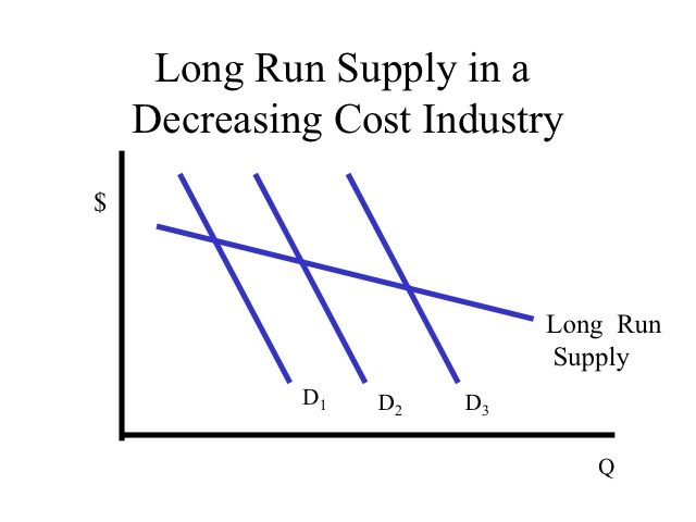
When both demand and supply curves are downward sloping:
This is seen in long-run supply curve in a decreasing cost industryWhen both the demand curve and the supply curve are downward-sloping, it is possible for them to have more than one point of intersection. For simplicity, we assume a situation where the supply curve is downward-sloping but is flatter (more horizontal) than the demand curve. In this case, there is a unique point of intersection of the curves and this gives the market price and equilibrium quantity traded.

Long Run Supply
Source: Refer this Link and Wiki

(UPSC Economics Optional 2014) Question 3:

Differentiate between the complete, partial and zero crowding out effect of a given increase in government expenditure in an economy.

  1. Definition: Crowding out refers to the situation when government must finance its spending with taxes and/or with deficit spending, leaving businesses with less money and effectively crowding them out.
  2. For better understanding of crowding effect:click here 


  3. If Crowding out is complete: Decrease in pvt spending is completely offset by govt spending financed by debt and there is no change in equilibrium.
  4. In Partial crowding out, there is a decrease in Private spending which partially offsets the multiplier effect from an increase in deficit-financed government spending. This causes AD1 to shift to AD'2 and E'2 is the new equilibrium instead of AD2 and E2( which is a zero crowding out position).
  5. Keynesian theory predicts  zero crowding out effect which means when Government expenditure increases by borrowing --> AD shifts from AD1 to AD2 while Consumption and Investment remain unaffected.
  6. The channel of its operation is :

  7. Source: Macroeconomics for Today, Tucker

Sunday, 21 December 2014

(UPSC Economics Optional 2014) Question No. 2


Explain the H theory of Money Supply.

Note: Unlike the first question, this one is straight forward and the answer can be found in any books Macro book by Ahuja, Jhingan or Monetary Economics book of S B Gupta. Surprisingly, the respective pages of SB Gupta's text are found here.

Answer:

Supply of money is policy determined.Hs = H. There is bar above H which means its exogenous to the public and banks.
Hd is the demand for H, which is the sum of the currency demanded by the public (C) and by banks as reserves (R).
C= c.DD
R= r.D---- (1)
TD= t.DD
D= DD+TD
   =(1+t) DD
(1) becomes R = r (1+t) DD

We have Hd = C + R = [c+ r( 1+t) ] DD
Hs = Hd implies,
H= [c+ r( 1+t) ] DD
From above,
DD= H/ [c+ r( 1+t) ] which is the equilibrium value of DD in terms of H and 1/ [c+ r( 1+t) ]  is called the demand- deposit multiplier.

We know Ordinary Money is M = C + DD = (1+c)DD = (1+c)H/[c+ r( 1+t) ] 
and the expression (1+c)/[c+ r( 1+t) ]  gives the money multiplier or m.

We have M =(1+c)H/[c+ r( 1+t) ]  which is rewritten as m. H 
M= m. H

Implications:
1. The monetary authority has to assume m as exogenously determined and that it will influence M.
2. m depends on behavioral choices of the public and banks.

Saturday, 20 December 2014

(UPSC CS Economics Optional 2014) Question No. 1

I am posting here the answer for the first question. You are most welcome to correct the answer and make additions wherever necessary by commenting below. I would be answering all the question in the coming days.
Q. No 1: Examine the relationship between own and cross price elasticities for a compensated demand function. (10 marks)
Own-price elasticity or simply price elasticity – shows the percentage rise in the demand at a percentage rise in the price of the good itself.
As the demand curves generally have a negative slope the own-price elasticity turns negative too, which corresponds to a decline in the demand when the price increases.
Cross-price elasticity shows the percentage increase in demand for good i as a result of a percentage increase in the price of good j. If there is a close substitution the cross-price elasticities will be positive as a price increase of good i will make the consumers substitute towards demanding good j. If i and j are complementary goods the cross-price elasticity will be negative.
Compensated demand curve: A compensated demand curve shows the relationship between the price of a good and the quantity purchased on the assumption that other prices and utility are held constant. The curve (which is sometimes termed a “Hicksian” demand curve) therefore illustrates only substitution effects. Mathematically, the curve is a two-dimensional representation of the compensated demand function.
 x=  xc ( px py, U)


Compensated own-price elasticity of demand (exc , px): This elasticity measures the proportionate
compensated change in quantity demanded in response to a proportionate change in a good’s own price

Compensated cross-price elasticity of demand (exc , px): This measures the proportionate compensated change in quantity demanded in response to a proportionate change in the price of another good.


is the required relationship.

Source: Microeconomic theory(10th Ed.), Walter Nicholson and Christopher Snyder